Introduction To Gradient descent algorithm (With Formula)

by keshav

---

---

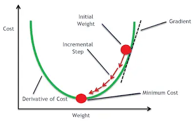
Gradient descent is a first-order iterative optimization algorithm for finding the minimum of a function (commonly called loss/cost functions in machine learning and deep learning). To find a local minimum of a function using gradient descent, one takes steps proportional to the negative of the gradient (or approximate gradient) of the function at the current point. If, instead, one takes steps proportional to the positive of the gradient, one approaches a local maximum of that function; the procedure is then known as gradient ascent. Gradient descent is also known as the steepest descent.

Before going through the variants of gradient descent let’s first understand how the gradient descent algorithm works. For this let’s take an example of the logistic regression model. For convenience, let’s suppose that our model has only two parameters: one weight w and bias b. For this the algorithm can be written as:

 

1. Initialize our w and b with random guesses. (e.g. say w=1, b=1).

 

2. Select a value for learning rate α. the learning rate is a factor that determines how big or small the step should be on each iteration. If the learning rate is too small, it would take a long time to converge and thus will be computationally too expensive. In the same way, if the value of the learning rate is too large, it will overshoot the minimum and fail to converge. 

 

3. The data should be normalized to a suitable scale if is highly varying. It will decrease the chances of error. There are various techniques of normalization. For their details about Normalization, you can visit this page.

 

4. Suppose our cost function/ loss function ( for brief about loss/cost functions visit here.) which is to be minimized be J(w,b). On each iteration, we take the partial derivative of cost function J(w,b) with respect to the parameters (w,b):

5. We then update our previous weight wand bias b as shown below:

6. We continue this process until the cost function converges.

Now let’s discuss in brief the variants of gradient descent algorithms.

 

• Batch Gradient Descent

It is also simply called gradient descent. In this algorithm, we consider all of our examples (whole data set) on each iteration when we update our parameters.

Update equation:

Advantages:

1. It has an unbiased estimate of gradient i.e. lower chances of error.
2. We can use a fixed learning rate during training for our entire example.

Disadvantages:

1. It takes a long time to converge if we have large data set.
2. It is computationally expensive.

 

• Mini-batch Gradient Descent

In this algorithm, instead of going through entire examples (whole data set), we perform a gradient descent algorithm taking several mini-batches. So even we have a large number of training examples, it is processed in batches of certain examples (batch size). We divide our data set into several mini-batches say n batches with certain batch sizes. 

The batch size can be tuned by us. Generally, it is chosen as a power of 2, examples 32, 64, 128, etc. It is done because some hardware such as GPUs achieves better runtime with batch size as a power of 2. 

Update equation:

Advantages

1. It is faster than the batch gradient descent.
2. Random selection of examples will help to avoid examples that are very similar and do not contribute much to the learning.

Disadvantages

1. Mini-batch requires the configuration of an additional “mini-batch size” hyperparameter for the learning algorithm.
2. Error information must be accumulated across mini-batches of training examples like batch gradient descent.

 

• Stochastic Gradient Descent

Stochastic gradient descent, often abbreviated SGD, is a variation of the gradient descent algorithm that calculates the error and updates the model for each example in the training dataset. In other words, can say it is a mini-batch gradient descent with batch size 1 and has batches equal to the number of training examples.

Update equation:

Advantages:

1. It is simple to understand and implement, especially for beginners.
2. This increases the model updates frequency that can result in faster learning on some problems.

Disadvantages:

1. Updating the model frequently can be computationally too much expensive in comparison to the above variants.
2. The frequent updates may result in a noisy gradient signal, that may cause the model parameters and turn the model error to jump around.

---